
Closer Look at Slopes
This article is here to help formulate differential equation from verbal description of a system using the idea of slope. Lets first visit the idea of two variables moving the same or opposite direction. In the following figure few systems are shown. When a variable \(x\) is changing another variable \(y\) is also changing according to \(y=f(x)\). On the left plot \(y=x\) shows \(y\) has value in the same direction as \(x\). That is why both side of \(y=x\) has same sign. If \(y\) has value in the opposite direction as \(x\) then a sign flip is necessary to reflect the fact. \(y=-x\) is such a system. \(y=e^x\) or \(y=e^{-x}\) has value in only one direction regardless of the value of \(x\). The left plot shows systems where change of \(y\) happens in the same direction as change of \(x\). If \(dx\) is +ve then \(dy\) is +ve. If \(dx\) is -ve then \(y\) is also -ve. Hence the slope is +ve.
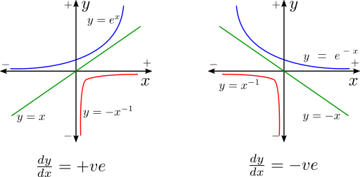
The right plot shows systems where change of \(x\) and \(y\) happens in the opposite direction. If \(dx\) is +ve then \(dy\) should be -ve and vice versa. Hence the slope is -ve. Othere than the direction of which way \(dx\) and \(dy\) changes relative to each other, the slope tells us something more insightful that can simplify a lot of equation formulation just by verbal description. It can also help us understand what an equation is doing which usually took me methods like drawing things, going both +ve and -ve directions to verify that the equation holds (for example diffusion equation). This insightful information is that the sign of the slope tells us the \(x\) or \(y\) direction in which \(y\) or \(x\) is increasing. The absolute value of the slope tells us how quickly \(y\) is increasing.
Using \(x\) direction
The sign of the slope tells us the \(x\) direction in which \(y\) is increasing and the absolute value of the slope tells us how quickly \(y\) is increasing. This is similar to how a gradient is defined. If \(\frac{dy}{dx}\) is +ve, it means \(y\) is increasing in the +ve \(x\) direction. If \(\frac{dy}{dx}\) is -ve, then \(y\) is increasing in the -ve \(x\) direction. This can be verified in the figure above.

Let us see how this interpretation helps us formulate equations. The leftmost plot in the figure above shows variation of \(\mathcal{L}\). If I have to find the \(x\) where \(\mathcal{L}\) is minimum iteratively, I must go in a direction where \(\mathcal{L}\) is decreasing. This direction is now easy to find. I must go in a direction opposite to the increase of \(\mathcal{L}\). Since \(\frac{d\mathcal{L}}{dx}\) gives me the \(x\) direction of increasing \(\mathcal{L}\) I must go \(-\frac{d\mathcal{L}}{dx}\) direction. Lets move \(\Delta{x}\) in that direction.
\[\Delta{x}\propto -\frac{d\mathcal{L}}{dx}=-\alpha\frac{d\mathcal{L}}{dx}\]This is known as the gradient descent. We can choose how much we want to move in that direction by choosing \(\alpha\). Without thinking like this I would have had to think what should be the case when slope is +ve and what for -ve slope seperately. But if I take slope as the \(x\) direction of increasing \(y\) then we can write the gradient desccet equation witout having to draw anything.
The middel plot describes the fact that there is a flow \(F\) happens in the direction where \(n\) is decreasing. If \(\frac{dn}{dx}\) indicates the \(x\) direction of increasing \(n\) then \(F\) must be in the direction if decreasing \(n\) i.e. \(-\frac{dn}{dx}\).
\[F \propto -\frac{dn}{dx} = -D\frac{dn}{dx}\]This is the condition for diffusion. The more the concentration gradient (difference of concentration) the more the flow and flow is in the direction of decreasing concentration.
The rightmost figure is similar to the diffusion. \(E\) is in the direction of decreasing \(V\). Lets use the gradient sign here for convenience.
\[E=-\nabla{V}\]This is the well known relationship between potential \(V\) and electric field \(E\). The reason \(E\) is in the direction of decreasing \(V\) is because to get any stored potential, work must be done in the direction against the electric field. As we go more against the electric field more potential energy is stored. Consequently, going in the direction of the electric field decreases the potential.
With these examples it should be easy to see how differential equation can be written just from the verbal description.
Using \(y\) direction
Above we defined a quantity using the slope. The defined quantity had the direction related to \(x\). That is why treating the slope sign in terms of \(x\) direction was helpful. If we have to relate the slope with the direction of \(y\) then treating the slope sign in terms of \(y\) will be helpful. The sign of the slope can be treated as the direction of \(y\) in which \(x\) is increasing. The absolute value of the slope indicates how fast \(y\) is changing just as was the case before. Previously we used slope to set a quantity. This time we will set the slope using other quantity. In other words we will define the dynamics of a quantity.

Leftmost plot in the figure above shows two traces. Top one has -ve slope and the bottom one has +ve slope. However, both of them are describing the same system. We will see how. First let us define a process by enforcing the way \(y\) changes. As the quantity \(x\) evolves (increases) \(y\) should go towards zero as fast as the value of \(y\). Under this condition what should the mathematical description of the proess or the evolution of \(y\) look like? The evolution is described by \(\frac{dy}{dx}\). Because \(y\) should go towards zero as \(x\) increases, we have to find the direction towards zero. The direction of zero is found by flipping the sign of any quantity. The direction towards zero for \(y\) is \(-y\). Hence the direction of \(y\) as \(x\) evolves should be \(-y\).
\[\frac{dy}{dx}\propto -y = \frac{-y}{\tau}\]\(\tau\) is there to fix the unit on both sides. It is now easy to see why both traces on the leftmost plot are describing the same process. Whatever the position of \(y\) is, it moves towards zero as \(x\) progresses. This is how a capacitor and resistor network or the RC network behaves. How fast \(y\) decreases depends on the inclination of the slope which is \(\mid-y\mid\). Hence, as \(\mid-y\mid\) smaller it gets slower in decreasing \(y\) and stops evolving when \(y\) gets to zero. Ideally and practically it never gets to zero because it gets so slow that it stops moving. If we manupulate the dyanmics by some external means for example by applying a stimulus \(S\), the dynamics \(\frac{dy}{dx}\) will be added effect of both \(-y\) and \(S\).
\[\frac{dy}{dx} = \frac{-y+S}{\tau}\]If \(S>y\) then the slope is +ve and \(y\) increases. But as \(y\) increases it gets closer to \(S\), \(-y+S\) gets smaller, increase of \(y\) slows down and stops moving as \(y\to{S}\). This effect is illustrated in the middle plot for \(S=\pm{a_0}\).
What if instead of setting \(\frac{dy}{dx}\) to the direction of zero we set it towards the direction of y? Whiche means as \(x\) evolves \(y\) changes in the direction of \(y\) hence we do not need the -ve sign.
\[\frac{dy}{dx}=\frac{y}{\tau}\]This is the description of +ve feedback sysstem. \(y\) becomes stronger and stronger as \(x\) progresses. The plot on the rightmost shows this process.