Differential Equations, Filters, Poles and Zeros

A constant coefficient first order ODE on the unknown \(y(t)\) and solution is of the form¹

\[\begin{align*} &\frac{dy}{dt} = ay + b \\ &\frac{d}{dt}(y + \frac{b}{a}) = a(y + \frac{b}{a}) \\ &\frac{\frac{d}{dt}(y+\frac{b}{a})}{y+\frac{b}{a}} = a \\ &\frac{d}{dt}(ln|y+\frac{b}{a}|) = a \\ &ln|y+\frac{b}{a}| = at + c \\ &y = \pm C e^{at} - \frac{b}{a}\\ \end{align*}\]

\(C\) is set by initial condition. For any ODE the solution can be given as \(y = y_c + y_p\). The solution can be thougth of as sum of solution to homogeneous equation (\(b=0\)), \(y_c\) (complementary function) and particular solution (stady state value of \(y\) when \(b\neq0\)) \(y_p\). For engineering application we set \(y(t)\) as response of a system and \(b\) as input. Then \(y_c = \pm C e^{at}\) is the natural response of the system when there is no input and \(y_p=-\frac{b}{a}\) is the effect of input \(b\) (stady state solution).

This system is also a filter (when \(b\) is time dependent). When a system’s property (like stability) needs to be analyzed, its transfer function in Laplas transtromed form tells us all the information wihtout even solving for a solution.

\[\begin{align*} &\frac{dy}{dt} = ay + b \\ &sY = aY + B \\ &H(s)=\frac{Y}{B} = \frac{1}{s-a} \\ &h(t) = e^{-at} \end{align*}\]

\(H(s)\) is the transfer function and also the impulse respose (as B(s)=1). Since any function can be composed of impulses, the convergence of impulse respose tells us about the stablity of the system. Here we can see for \(h(t)\) to converge at \(t\to \infty\), the pole needs to be on the left hand side of s-plane.

Lets take a look at simplest form of low and high pass filter.

‍ \(\begin{align*} &\tau\frac{dy}{dt} = -y + b \\ &\tau sY = -Y + B \\ &H(s) = \frac{1}{\tau s+1} \\ &H(s) = \frac{\omega_c}{s+\omega_c} \\ &h(t) = \frac{1}{\tau}e^{-\frac{t}{\tau}} \\ \end{align*}\)

‍ \(\begin{align*} &\tau\frac{d}{dt}(b-y) = y \\ &\tau\frac{dy}{dt} = -y + \tau\frac{db}{dt} \\ &\tau sY = -Y + \tau sB \\ &H(s) = \frac{\tau s}{\tau s+1} \\ &H(s) = \frac{s}{s+\omega_c} = 1-\frac{\omega_c}{s+\omega_c} \\ &h(t) = \delta(t) - \frac{1}{\tau}e^{-\frac{t}{\tau}} \\ \end{align*}\)

This sentence is invisible to make two columns to have same number of lines so that anyting appearing below appears properly bla bla bla bla Right away we can link some charactaristics from the differential equation to the pole and zero of the system.

1. poles arise from \(\frac{dy}{dt}\) time constant and zeros arise from \(\frac{db}{dt}\) time constant
2. pole is on the left hand side if \(\frac{dy}{dt}\propto -y\), on the right hand if \(\frac{dy}{dt}\propto +y\)
3. highpass zero does not have the form \((\tau s + 1)\) because there is no \(-b\) term.

In general for a system modeled by differential equation

\[\begin{align*} &a_n\frac{d^ny}{dt}+a_{n-1}\frac{d^{n-1}y}{dt} + \cdots + a_1\frac{dy}{dt} + a_0y = b_m\frac{d^mx}{dt}+b_{m-1}\frac{d^{m-1}x}{dt} + \cdots + b_1\frac{dx}{dt} + b_0x \\ &a_ns^nY(s)+a_{n-1}s^{n-1}Y(s) + \cdots + a_1sY(s) + a_0Y(s) = b_ms^mX(s)+b_{m-1}s^{m-1}X(s) + \cdots + b_1sX(s) + b_0X(s) \\ &H(s) = \frac{b_ms^m+b_{m-1}s^{m-1} + \cdots + b_1s + b_0}{a_ns^n+a_{n-1}s^{n-1} + \cdots + a_1s + a_0}\\ &H(s) = \frac{N(s)}{D(s)} = K\frac{(s-z_1)(s-z_2)\cdots(s-z_m)(s-z_{m-1})}{(s-p_1)(s-p_2)\cdots(s-p_n)(s-p_{n-1})} \end{align*}\]

\(K=\frac{b_m}{a_n}\) is the gain of the filter/amplifer.

• For the first order case pole/zero came directly from the time constant of the capacitor. But for higher order case the time constants of all the capacitors(or inductors or spring i.e any energy storage element) combine together to form poles and zeros.
• The poles come from \(y\) side’s coefficient and zeros come from \(b\) side’s coefficients.
• The system is stable if the natural response \(y_c\) (homogeneous solution) is convergent. Which means when there is not any external excitation, the system response will decay from the value any previous excitation leaves behind. When all the \(b\)’s are zero on the right hand side of the differential equation, The homogeneous solution is given by the system poles

\[\begin{align*} &a_n\frac{d^ny}{dt}+a_{n-1}\frac{d^{n-1}y}{dt} + \cdots + a_1\frac{dy}{dt} + a_0y = 0 \\ &a_ns^nY(s)+a_{n-1}s^{n-1}Y(s) + \cdots + a_1sY(s) + a_0Y(s) = 0 \\ & a_ns^n+a_{n-1}s^{n-1} + \cdots + a_1s + a_0 = D(s) = 0 \\ &(s-p_1)(s-p_2)\cdots(s-p_n)(s-p_{n-1}) = 0 \\ &y_c(t) = \sum_{i=1}^nC_ie^{p_it}\\ \end{align*}\]

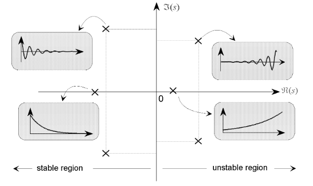
The homogeneous solution/unforced response is given entirely by \(D(s)\) or the system poles and \(N(s)\) is not needed. And for \(y_c(t)\) to converge poles must be on the left hand side in s-plane. This way time domain impulse response is not needed and saves us calculation involving zeros and factorization. \(C_i\) are subject to initial conditions. The image below (taken from²) shows the effect of pole location on the unforced response.

s-plane and H(s)

Reason why Laplas tranformation or Fourier transformation is handy is because of eigenvalue/eigenfunction property. It makes calculation a lot easier if the output is just a scaled and/or shifted version of the input.

‍\(x(t) = e^{st} \\ y(t) = \int_{-\infty}^{+\infty} h(\tau)x(t-\tau)d\tau \\ y(t) = \int_{-\infty}^{+\infty} h(\tau)e^{s(t-\tau)}d\tau \\ y(t) = e^{st}\int_{-\infty}^{+\infty} h(\tau)e^{s\tau}d\tau \\ H(s) = \int_{-\infty}^{+\infty} h(\tau)e^{s\tau}d\tau \\ y(t) = H(s)e^{st}\)

‍\(x(t) = \int_{-\infty}^{+\infty}X(s) e^{st}ds\\ y(t) = \int_{-\infty}^{+\infty} H(s)X(s)e^{st}ds\\\)

This sentence is invisible to make two columns to have same number of lines so that anyting appearing below appears properly bla bla bla bla This sentence is invisibl

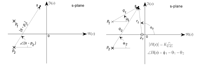
If the input is exponential function then output of the system is just the input exponential scaled by \(H(s)\) which introduces scale factor and shift (if \(H(s)\) is complex). \(e^{st}\) is eigenvector and \(H(s)\) is eigenvalue³. Just like fourier transfrom, any signal is linear sum of periodic signals (complex exponentials \(e^{j\omega t}\)) but this time the periodic signals have decaying/exploding factor \(e^{\sigma t}\) to help with convergence issue faced by fourier transform. If we know what \(s\) components make up \(x(t)\), we can find the output by just scaling each \(s\) components by system response \(H(s)\) and add/integrate them together. So in a s-plane like as blow, when \(H(s)\) is being evaluated at a point, it means evaluating system response for that \(s\) component.

For frequency response (Bode plot) we need only sinosoidal component response. Hence \(H(s)\) will be only evaluated on the imaginary axis for frequency response.

Effect of zero in stability

We have seen for stabilty we only need system poles. But what if the input itself is unbounded? The effect of input is represented by the zeros. So zero should also affect stability in some way. Right hand side zero causes some stability problem as seen in Miller compensation. Explanation?!

---

1. Ordinary Differential Equations, Gabriel Nagy ↩

2. Understanding Poles and Zeros ↩

3. Signals and Systems by Oppenheim, Willsky, 2nd Edition, pp.182 ↩