Feedback Sytem

Feedback system is an important concept in engineering priciples. A good uderstanding of the process helps build intuition of any process involving feedback and helps predict the outcome without going through difficult calculations. This page documents how I came to understand feedback system as a pysical process.

A typical feedback system is illustrated as following figure. This is a negative feedback system. Part of the output is fed back to the input which reduces the total input that goes into the whole system. A puls sign would mean it is a positive feedback system. Part of the output is fed back to the input that adds on top of the existing input and goes as input into the whole system.

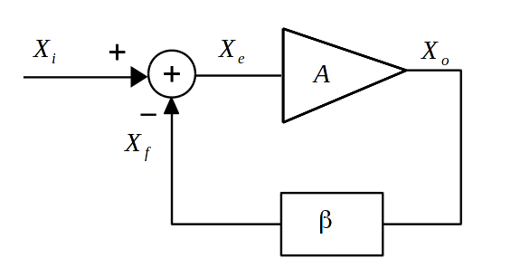
The error signal \(X_e = X_i - X_f\) is the input to the main process with gain \(A\) having transfer function \(X_o = AX_e\). Part of the output is fed back using feedback transfer function \(X_f = \beta X_o\). \(X_f\) is subtracted from \(X_i\) to create new input and the process keeps repeating. For the system to be stable the error signal \(X_f\) has to be the same as it started out with. This way after \(X_e\) passes though \(A\) and \(\beta\) and comes back again it produce the same value of \(X_e\) so the system does not go into unstability. The stable output can be derived from this argument.

\[\begin{align} X_e &= X_i - A\beta X_e \nonumber \\ X_e &= \frac{1}{1+A\beta}X_i \nonumber \\ X_o &= AX_e = \frac{A}{1+A\beta}X_i \nonumber \end{align}\]

When the system starts, it cannot have the exact value of $X_e$ needed for stable output. So the system output goes back and forth and searches for a stable point utill it converges to a stable output. So the feedback will have some transient response before it can settle to a stable output because there are competing force from input to output and from output to input that keeps changing the input to the forward path. These two force are governed by two equations.

\[\begin{align} X_o &= AX_e \\ X_e &= X_i - \beta X_o \nonumber \\ X_o &= \frac{X_i}{\beta} - \frac{1}{\beta}X_e \end{align}\]

The system converges to the solution of these two system of equations. The intersection of the two lines gives us the operating point of the system.

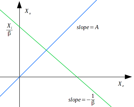
Now we can pretty much see how the system can go into something other than stable points or in other words unstability. If the two lines are parallel then there is no intersection. Which means if slope the lines are equal \(A = -1/\beta\) or \(A\beta = -1\) the system will go into unstability.

I think it is essential to also understand what happens pysically in the process that can make the system settle to a stable position or drive it to unstability. To understand this lets see what happens every time the output loops though. Lets assume the initial output when the system starts is zero. Then

\[\begin{align} 1st \quad iteratoin: X_e &= X_i \nonumber \\ 2nd \quad iteratoin: X_e &= X_i - A\beta X_i \nonumber \\ 3rd \quad iteration: X_e &= X_i - A\beta X_i + (A\beta)^2 X_i \nonumber \\ 4th \quad iteration: X_e &= X_i - A\beta X_i + (A\beta)^2 X_i - (A\beta)^3 X_i \nonumber \end{align}\]

We can see that it is implementing a power series. Also \(X_e\) is acting like an accumulator. In every iteration \(X_e\) is scaled by \(A\beta\) and adds in \(X_i\) to produce new \(X_e\). Much like in programing language.

int Xe = 0;
for (int i=0;i<LIMIT;i++)
{
    Xe = -A*b*Xe + Xi;
}

In this case however it will be looping infinite times. In that case for the power series to converge it must be \(|A\beta| < 1\). \(|A\beta| >=1\) makes the power series to grow without bound and drives the system into unstability. This result is also obtained considering the slope the lines. (further on slopes will be written later).