Ocean Scripting

How to open OCEAN prompt in UNIX shell?

For this you need to load necessary paths to your environment variable. I found it easy to turn startcad script into a script for starting the OCEAN prompt. In the startcad script delete the lines associated with DRC/LVS settings. Replace the line containing virtuoso & with ocean. Save it with a suitable name for example startocean. Open a UNIX shell, go to the directory containing startocean and run these commands.

$ chmod 755 startocean
$ ./startocean

The UNIX shell should turn into an OCEAN shell.

---

Creating Netlist files

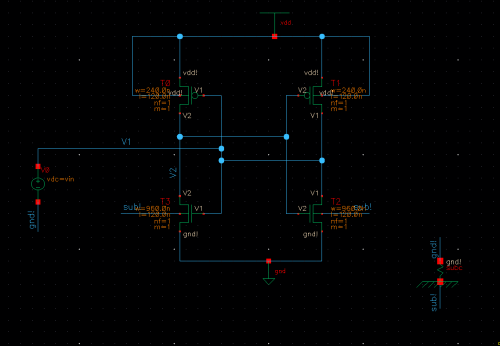
There is a hard way to make netlist files for simulation that generates netlist from schematic and additional formatting needs to be done by hand. But the easiest way is to use the ADE window for simulation. Set the ADE window for some basic simulation (ex. tran or ac) and save the session. This will create the netlist in the library directory. But before that lets draw this SRAM circuit. We will be plotting butterfly curve using OCEAN scripting.

Optionally you may need to create another file listing the necessary stimulus if there is any stimulus in the circuit. In this case we have a stimulus. This node vdd! which needs to be set at a voltage (same as setting global stimuli in the ADE simulation window → Setup → Stimuli). So create another file containing this line.

_vvdd! (vdd! 0) vsource dc=1 type=dc

Save it with .scs extension for example _graphical_stimuli.scs in the same directory as the netlist. If there were no stimulus in the circuit there would have been no need to declare a stimulus file. For example if we replaced vdd with a voltage source vdc there is no need for stimulus file.

Create and Run OCEAN Script

Now open a text file and fill it with these lines. This shows the general structure of the simulation setup

;;;=========================================== set simulator ==============================================;;;
simulator( 'spectre )

;;;=========================================== netlist design ==============================================;;;
design(	 "/home/username/cadence/scripting/butterfly_plot/netlist")

;;;========================================= resutls directory =============================================;;;
resultsDir( "/home/username/cadence/scripting/Results" )

;;;========================================= library model files ===========================================;;;
modelFile( 
    '("/home/username/cadence/practice/models/allModels.scs" "tt")
    '("/home/username/cadence/practice/models/design.scs" "")
)

;;;========================================= stimulus file if any ===========================================;;;
stimulusFile(?xlate nil "/home/username/cadence/scripting/_graphical_stimuli.scs")

;;;==================================== Any parameter initialization ========================================;;;
desVar("vin" 0)

;;;=================================== Analysis type - tran, dc,ac ==========================================;;;
analysis('dc ?param "vin" ?start "0" ?stop "1" ?step "0.01"  )

;;;================================ Environment option - analysis order =====================================;;;
envOption(
	'analysisOrder  list("dc") 
)

;;;=========================================== set temperature ==============================================;;;
temp( 27 ) 

;;;============================================ save current data ===========================================;;;


;;;================================ run simulation, select result, plot =====================================;;;
run()
selectResult( 'dc )
ocnYvsYplot(?wavex v("V1") ?wavey v("V2"))
ocnYvsYplot(?wavex v("V2") ?wavey v("V1"))

In the code, anything after ; is a comment. Replace the design netlist path, stimulus file path, library with the paths to your files. Save it with .ocn extension for example butterfly.ocn. Place the .ocn file in the same directory as startocean file directory. Now in the OCEAN shell run this command.

load "butterfly.ocn"

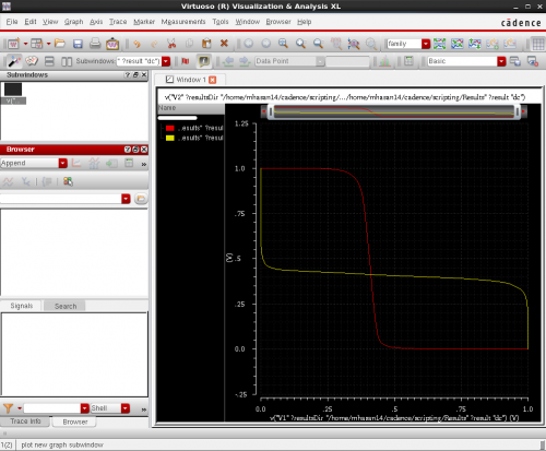
A butterfly plot should be shown like in the figure.

Now In the code, there is a section named save current data. This section is required if you want to plot device currents as well. Spectre does not save currents by default. You need to tell spectre to save currents by this command.

save('alli)

Now if you run the command outputs() in the OCEAN shell it will output the waveform names/nodes that it saved. You can use those names to plot the currents.

Note: I don’t know when ocnYvsYplot was introduced in OCEAN. It was not available in 4.4.6 version. I have found it in the OCEAN Reference Product Version 5.1.41 June 2004. Our current product version is 6.1.6.

---

Using OCEAN to choose design parameters

OCEAN scripting is a useful tool to choose design parameters by varying those parameters and checking if some values meets design requirements. Say for example we want to know what should be the width and length of transistors in an inverter that is driving a 5.0fF capacitor, to achieve a delay of less than 8.0ps?

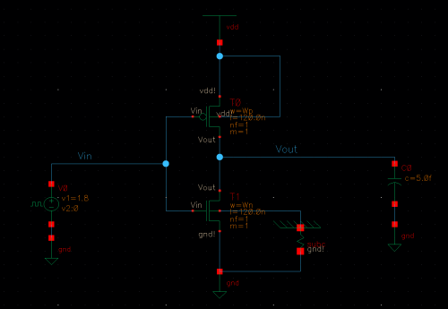
By setting various values of the widths and heights of the inverter transistors and each time checking the delay between input and output we can have an estimate of our desired Wp and Wn. We can use programming constructs like while loop to do this in OCEAN script. Although ADE window is able to perform parametric simulation but a user has no control over when to do something if a desired condition appears. Furthermore it is also possible to track every moment of the simulation and log it a text file. You can even save a plot as image at some desired point of simulation. A simple code for this is given below. This sweeps values of Wp and Wn and on each swipe delay is calculated. If it meets the design requirements (delay below 8.0ps) the the loop is terminated and an image of plot for minimum delay is saved for observation. On each swipe delay values for each Wp and Wn is also written to a text file named print_delay.txt It also saves an image of the desired delay plot.

;;;=========================================== set simulator ==============================================;;;
simulator('spectre)

;;;=========================================== netlist design ==============================================;;;
design("/home/mhasan14/cadence/scripting/delay_inv/netlist")

;;;========================================= resutls directory =============================================;;;
resultsDir("/home/mhasan14/cadence/scripting/Results")

;;;========================================= library model files ===========================================;;;
modelFile( 
    '("/home/mhasan14/cadence/scripting/models/allModels.scs" "tt")
    '("/home/mhasan14/cadence/scripting/models/design.scs" "")
)

;;;========================================= stimulus file if any ===========================================;;;
stimulusFile(?xlate nil
	"/home/mhasan14/cadence/scripting/delay_inv/_graphical_stimuli.scs"
)

;;;==================================== Any parameter initialization ========================================;;;
desVar("Wp" 480n)
desVar("Wn" 160n)

;;;=================================== Analysis type - tran, dc,ac ==========================================;;;
analysis('tran ?stop "5n")

;;;================================ Environment option - analysis order =====================================;;;
envOption(
	'analysisOrder  list("tran") 
)

;;;=========================================== set temperature ==============================================;;;
temp(27)

;;;============================================ save current data ===========================================;;;
save('all)

;;;================================ run simulation, select result, plot =====================================;;;

;;;========================================= opens a text file ==========================================;;;
out = outfile("print_delay.txt")

;;;====================================== control using while loop =======================================;;;
designWp = 0
designWn = 0
designDelay = 8p
minD = 0;

wp = 160n
while(wp <= 960n
     desVar("Wp" wp)

     wn = 160n
     while(wn <= 960n
           desVar("Wn" wn)
           run()
           selectResult( 'tran )
           plot(v("Vout") )
     
	   d = delay(?wf1 v("Vin") ?value1 1.0 ?nth1 2 ?edge1 'rising 
                     ?wf2 v("Vout") ?value2 1.0 ?nth2 2 ?edge2 'falling )
           fprintf(out "delay for Wp=%3.15f and Wn=%3.15f is %3.15f\n", wp, wn, d)
	   if(d < designDelay then

		designWp = wp
		designWn = wn
                a = v("Vout")
                minD = d
           else
             nil
           )
           
           wn = wn + 200n
     )
	wp = wp + 200n
)
fprintf(out "\n delay is minimum for Wp=%3.15f and Wn=%3.15f with minimun delay %3.15f\n", designWp, designWn, minD)
close(out)

newWindow()
plot(v("Vin") a)
;;;========================================= save a png file ==========================================;;;
hardCopyOptions(?hcOutputFile "minDelayPlot.png")
hardCopy()

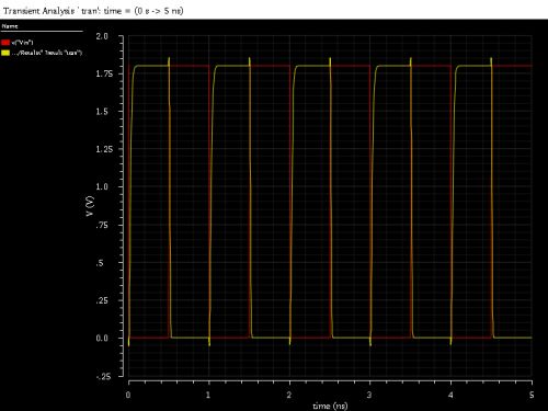
The resulting plot looks like the figure on the right. The .png file will be created in the same directory as the .ocn scripting directory.